Spot lead pricing II: The fishy distribution
When I worked in media analytics / campaign management, when a statistic was to be reported on was that 'things' were drawn from the Normal distribution. The general arm-wavy argument was along the lines of "... mumble mumble law of large numbers mumble burp ...". Of course, what they really intended to invoke was the central limit theorem. But hey, I too went to business school and understand that MBA level probability & statistics is dull and arm-wavy and hence was a great time to catch up on sleep, so I usually let that slide. In lay terms the argument is that we don't really need to know the underlying distribution because with enough samples, things look normal. In the world of media analytics, where we had billions of ad impressions and millions of clicks, the 'enough samples' part usually held. But in the world of lead-gen, where a single supplier may only provide 5 to 25 leads per day, this doesn't hold.
What distribution do I use to model leads arriving into an exchange? The Poisson distribution. If anyone remembers their probability classes from school, they will remember countless examples which invariably involved people arriving to a queue at a bank teller. If you happened to take computer science, the example might be expressed as jobs arriving at a CPU, or something like that. Either way one of the key measures to describe these processes is to state the average time between successive arrivals. If you can make the assumption that the process is memoryless, i.e., the time of arrival of the next person does not depend on the time of arrival of previous persons, then you can model the time between arrivals as an Exponential distribution. And if you do this the total number of people arriving over a time interval T is distributed as the Poisson distribution.
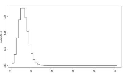 In the chart above we see a the distribution of the number of expected arrivals in one day, when the average time between arrivals is 4.8 hours (one fifth of a day). We can see that the we expect about 5 arrivals in the day, which should be blindingly obvious.
 The big difference is that unlike a normal distribution, a Poisson will have P(X < 0) = 0. In other words the chance of having a negative number of arrivals is zero. So, if you permit my own arm-waviness, the Poisson distribution is somewhat like the discrete analog of the LogNormal.
In my previous post I made the statement that a supplier providing a large number of leads was unlikely to supply a dramatically lesser number in the future. Lets examine the chance of a supplier providing exactly zero leads if the previously provided X leads per day. In R, we express this as
(I wish I could embed LaTeX in this blog...)
The Poisson probability distribution function is P(x) = l^x exp(-l/x!), where l is the mean number of arrivals and x is the number of arrivals that we want to know the probability of. If we set x=0 we get P(0) = l^0 exp (-l/0!) = exp(-l). So the chance of getting zero leads follows an exponential distribution and we are right back where we started this detour into the fishy distribution.
And as an exercise to the reader (don't you hate it when people do this..), what does the following mean in the context of lead gen?

What distribution do I use to model leads arriving into an exchange? The Poisson distribution. If anyone remembers their probability classes from school, they will remember countless examples which invariably involved people arriving to a queue at a bank teller. If you happened to take computer science, the example might be expressed as jobs arriving at a CPU, or something like that. Either way one of the key measures to describe these processes is to state the average time between successive arrivals. If you can make the assumption that the process is memoryless, i.e., the time of arrival of the next person does not depend on the time of arrival of previous persons, then you can model the time between arrivals as an Exponential distribution. And if you do this the total number of people arriving over a time interval T is distributed as the Poisson distribution.
 In the chart above we see a the distribution of the number of expected arrivals in one day, when the average time between arrivals is 4.8 hours (one fifth of a day). We can see that the we expect about 5 arrivals in the day, which should be blindingly obvious.
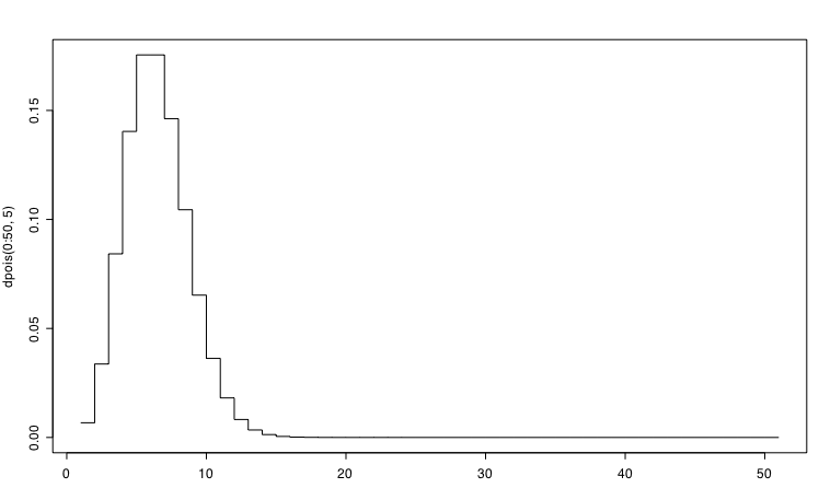
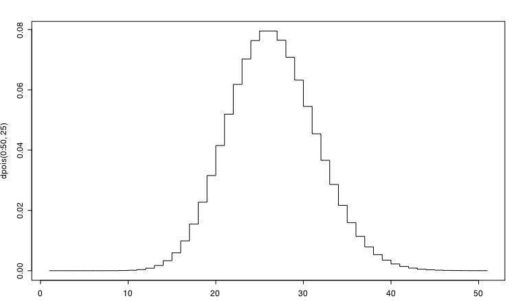
I'm very fond of the R statistical programming environment. It managed to get me through my statistical arbitrage course, while I profited from the arbitrage between S-Plus ($$$) and R (FREE!). To my untrained eyes, they are pretty similar.If you make arrival times more frequent, we end up with a distribution that looks like a discrete version of the Normal distribution:
To product the chart above in R:plot(dpois(0:50, 5), type='s')
 The big difference is that unlike a normal distribution, a Poisson will have P(X < 0) = 0. In other words the chance of having a negative number of arrivals is zero. So, if you permit my own arm-waviness, the Poisson distribution is somewhat like the discrete analog of the LogNormal.
In my previous post I made the statement that a supplier providing a large number of leads was unlikely to supply a dramatically lesser number in the future. Lets examine the chance of a supplier providing exactly zero leads if the previously provided X leads per day. In R, we express this as
plot(dpois(0, 0:50), type='s')I won't spoil the surprise ending by including the chart, but needless to say if you provide less leads you are more likely to provide zero leads. Mathematics is wonderful for stating the obvious, but humor me here.
(I wish I could embed LaTeX in this blog...)
The Poisson probability distribution function is P(x) = l^x exp(-l/x!), where l is the mean number of arrivals and x is the number of arrivals that we want to know the probability of. If we set x=0 we get P(0) = l^0 exp (-l/0!) = exp(-l). So the chance of getting zero leads follows an exponential distribution and we are right back where we started this detour into the fishy distribution.
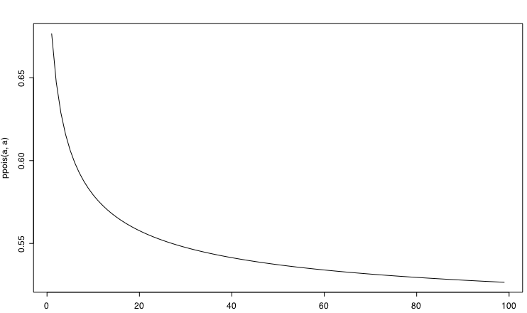
And as an exercise to the reader (don't you hate it when people do this..), what does the following mean in the context of lead gen?
a=2:100
plot(ppois(a,a),type='l')
posted by Joshua Reich at
8/02/2006 08:05:00 AM
![]()

2 Comments:
You could always use a kernel estimator to draw the distribution.
Jon -- when will you learn, if its not on Mathworld, its not Math!
Post a Comment
Subscribe to Post Comments [Atom]
<< Home